Estimating π using the State monad in Scala
In an attempt to better understand the State monad in Scala I wanted to do
something practical with it. One thought that came to mind was a simple Monte
Carlo simulation to estimate the constant π.
To estimate π using a Monte Carlo
simulation we can randomly
sample x and y values within a square centered around 0 to see if
they land inside r^2. If x^2 + y^2 <= r^2 then the point is inside of the
circle. We can then plug this amount into the formula for the ratio of the
area of a circle enclosed in a square which is:
If we solve for π using our simulation result as the ratio of the area we get:
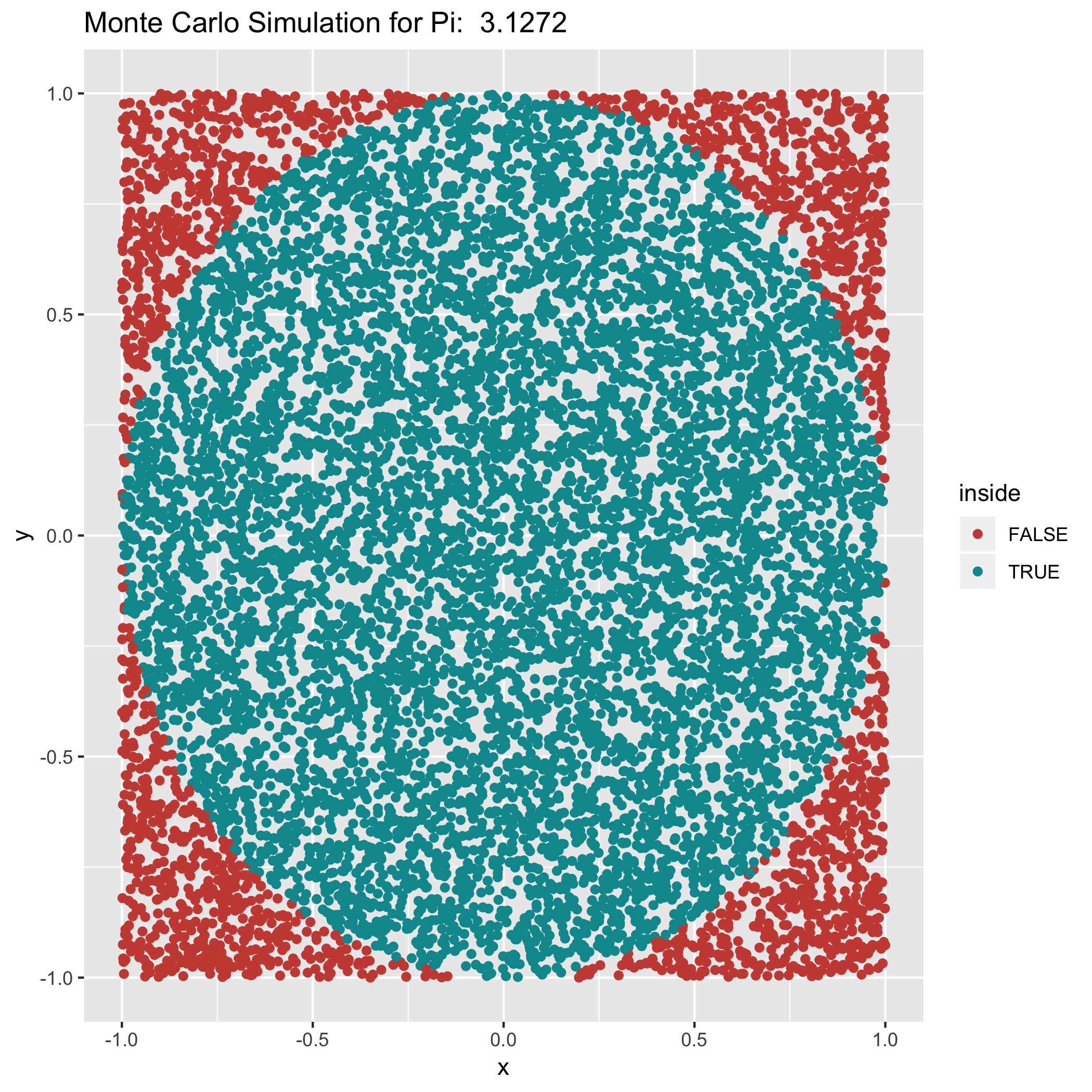
\[estimate \times 4 = \pi\]Let’s illustrate this random sampling for the ratio of points within the circle graphically in R:
set.seed(42)
runs = 10000
xs = runif(runs, min=-1, max=1)
ys = runif(runs, min=-1, max=1)
inside = xs^2 + ys^2 <= 1
df = data.frame(x=xs, y=ys, inside=inside)
estimate = sum(inside)/runs*4
ggplot(df, aes(x=x, y=y, color=inside)) +
    geom_point() +
    scale_color_hue(l=50) +
    labs(title=paste('Monte Carlo Simulation for Pi: ',estimate))
This gives us a plot of the circle with the random points that fell inside the differentiated from those that fell outside:
When I started thinking about this problem I was a little stumped regarding
how to feed a pure random number generator through a Scala for
comprehension while also accumulating the number of points within the circle.
I wanted to be able to pull a pair of x and y values from a pure random
number generator using a for comprehension to describe the simulation. I
was imagining something like the following:
for {
    x <- nextDouble
    y <- nextDouble
    isInCircle = (x * x + y * y) < 1.0
}
But I wasn’t sure how to accumulate the rolling ratio of coordinates within the unit circle. With a little help from Stackoveflow I was able to sort it out.
Once I got some help from SO, I had the pieces I needed to put it together.
The first piece we’ll need is a pure random number generator. We’ll call it
RNG:
object RNG {
  type RNG[A] = State[Long, A]
  def nextLong: RNG[Long] =
    State.modify[Long](
      seed => (seed * 0X5DEECE66DL + 0XBL) & 0XFFFFFFFFFFFFL
    ) >> State.get

  def nextInt: RNG[Int] = nextLong.map(l => (l >>> 16).toInt)

  def nextNatural: RNG[Int] = nextInt.map { i =>
    if (i > 0) i
    else if (i == Int.MinValue) 0
    else i + Int.MaxValue
  }

  def nextDouble: RNG[Double] = nextNatural.map(_.toDouble / Int.MaxValue)

  def runRng[A](seed: Long)(rng: RNG[A]): A = rng.runA(seed).value

  def unsafeRunRng[A]: RNG[A] => A = runRng(System.currentTimeMillis)
}
The key method for the purpose of generating random numbers for our Monte
Carlo simulation is the nextDouble method. This is what we’ll use to
generate a pair of x and y values.
The real insight from the SO post is the step function which allows us to
accumulate the rolling ratio of coordinates within the circle. We’ll break
out of our iteration or continue by signalling with Right or Left values
respectively. This is handled for us via the
tailRecM
function on the Monad trait in cats.
With nextDouble and the step pattern we can now implement our simulator:
case class Step(count: Int, inCircle: Int)

def calculatePi(iterations: Int): RNG[Double] = {
  def step(s: Step): RNG[Either[Step, Double]] =
    for {
      x <- nextDouble
      y <- nextDouble
      isInCircle = (x * x + y * y) < 1.0
      newInCircle = s.inCircle + (if (isInCircle) 1 else 0)
    } yield {
      if (s.count >= iterations)
        Right(s.inCircle.toDouble / s.count.toDouble * 4.0)
      else
        Left(Step(s.count + 1, newInCircle))
    }

  Monad[RNG].tailRecM(Step(0, 0))(step(_))
}
I put everything together in a repo on github. To run it:
sbt -warn "run 100000"
Estimated 3.14916 for Pi after 100000 iterations.
[success] Total time: 2 s, completed
Though the State monad is fairly simple on the surface there’s a lot going
on underneath in cats. For example, a naive implementation of
State.flatMap would not be able to support 10,000 iterations of our
simulation because it’s not stack safe. The for comprehension would create
nested instances of flatMap that would eventually exhaust the call stack.
The tailRecM method enables stack-less recursion for monads on the JVM. If
you’re interested in learning more see this
paper by Rúnar
Bjarnason. He’s one of the authors of Functional Programming in
Scala.
As a final thought, you may be thinking that there are easier ways to estimate π and you would be right. One of the insights that came out of the Basel Problem from Euler is a series that can be use to estimate π. In R it looks like:
s = seq(1, 10000)
sqrt(sum(1/s^2)*6)
[1] 3.141497
Or in Scala:
Math.sqrt((1 to 10000).foldLeft(0.0)((t, x) => t + 1/Math.pow(x, 2))*6)
res1: Double = 3.1414971639472147
I’m sure there are others.